6.1 Completion Optimization - Economics Input Calibration Tool
Guide to PetroVisor Economic Input Calibration Tool
Overview
Access the PetroVisor Economics Input Tool.
The Economic Input Calibration Tool is used in the Completion Optimization App and the A&D App.
The goal of the calibration tool is to determine the value of various economic inputs to match an observed average-well monthly operating cost. The tool summarizes the observed and model (calibrated) monthly operating costs and the difference between the two. The calibration process is iterative and can usually achieve a model/observes difference of less than 5% in a matter of minutes.

The calibration process has four steps:
- Enter initial economic inputs and observed production rates
- Calibrate the operating cost model
- Calibrate the NGL model
- Enter the economic inputs into PetroVisor
Once calibrated, the economic inputs are entered into PetroVisor in the Economics Parent Static Signal filter under the Data tab.
Enter Initial Economic Inputs and Observed Production Rates
The economic inputs are found in the ”Inputs” tab and are grouped into categories. The user can enter and change values in the grey-shaded cells and make selections in the dropdown boxes.
In the first section, enter information about the area under evaluation. The economic inputs may be different for different areas and different formations. This information allows multiple users to understand the area of application for these economic inputs.


Reversionary working interests can be modeled for both exiting wells and drilling locations. For existing wells, the user will typically assign a payout balance. Notice that entering a number greater than zero for “Payout Reversion Balance” causes the “Payout Multiple” to be greyed out. To utilize a Payout Multiple for reversion, either delete or enter zero for “Payout Reversion Balance” and enter the desired multiple of payout to trigger reversion.

Initial capital is usually intended for drilling/completion or rework capital expenditures.

The severance and ad valorem taxes vary by state and county.
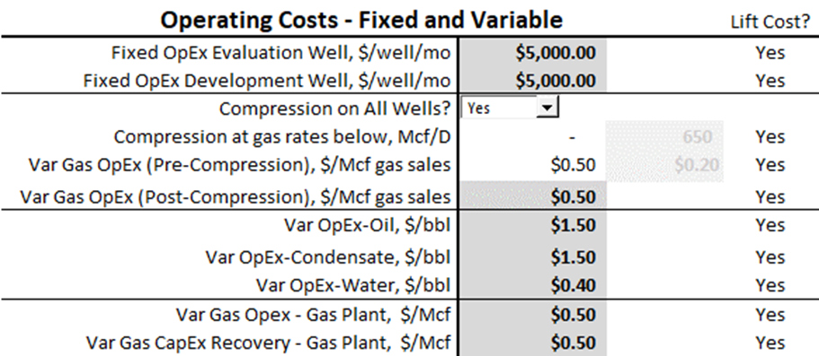
The operating costs may be sourced from accounting data, a reserves database, or estimates based on local experience. If these inputs need to be calibrated, enter reasonable initial values, and the calibration process will refine those numbers (discussed later in this article).
The user can impose production rate-triggered compression costs:
- If this feature is not needed:
- Select “Yes” in the “Compression on All Wells?” dropdown box
- The “Post-Compression” variable gas operating cost will be used for all wells.
- For production rate-triggered compression costs:
- Select “No” in the “Compression on All Wells?” dropdown box
- Enter the gas production rate that triggers the Post-Compression variable gas operating cost (used for months where a well’s average production is below this rate)
- Enter the Pre- and Post-compression variable gas operating costs
The user can also apply gas processing plant costs:
- Variable Gas OpEx
- Var Gas CapEx Recovery
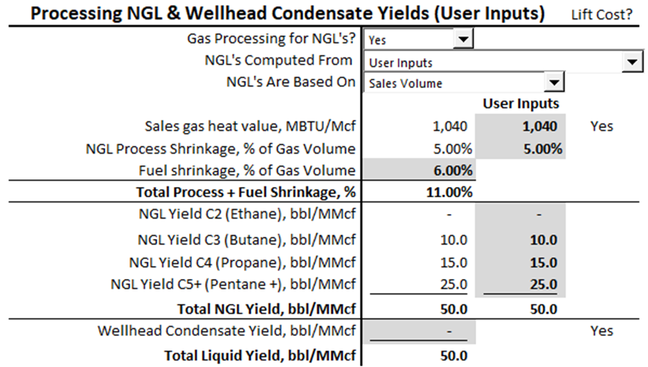
The NGL inputs may be sourced from accounting data, a reserves database, or local knowledge. If from local knowledge these inputs usually need to be calibrated to observed data.
The NGL inputs can be turned on or off by selecting “Yes” or “No” in the “Gas Processing for NGL’s?” dropdown list. When turned off, the NGL yields are set to zero and the user enters the sales gas heating value and gas shrinkage due to any fuel requirements, usually to run compressors.
Regardless of the NGL model being on or off, the user also enters a wellhead condensate yield that is additive to, and separate from, the NGL yield.
When turned on the model offers three options to compute NGL yields, gas shrinkage, and sales gas heating value with increasing degrees of sophistication. These models are selected from the “NGL’s Computed From” dropdown list:
- User Inputs
- User Inputs + Plant Type:
- Gas Analysis + Plant Type
If the NGL model is turned on and NO calibration is required (i.e. the user already knows the NGL component yields, sales gas heating value, and process/fuel gas shrinkage), then choose the “User Inputs” model and enter values into the grey shaded cells.
If calibration is required, the calibration process is discussed later in this article in the “Calibrate the NGL Model” section.

Wellhead condensate often contains small amounts of the lighter NGL components. If the condensate is being fractionated, the user can replicate the fractionation process by entering a % for each component in the “Condensate Composition” section. Ensure that the component %’s total to 100%. These purity products will be added to any NGL-derived purity products. If no fractionation, then set the C5+ % to 100.
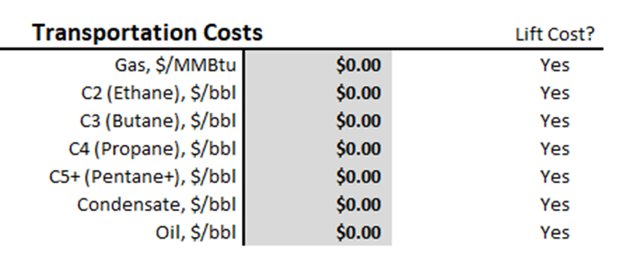
Transportation costs are intended to reflect local gathering & pipeline fees that are not included in the fixed and variable operating costs. They are included in the operating costs but can be turned off. Enter as positive numbers.
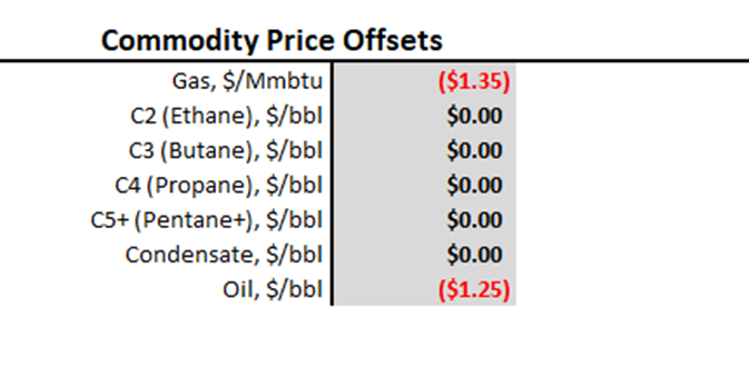
The Commodity Price Offsets are a basis differential between the hub commodity price being used in economic runs and the price received at the wellhead or custody transfer point. Offsets can be positive or negative.
Calibrate The Operating Cost Model
The fixed and variable operating costs, along with several other inputs, are intended to provide an overall single-well operating cost that matches observed data. In this calibration process, the user enters a target lifting cost ($/BOE/D) and production rates to compute an average-well monthly operating cost. The user then alters several operating cost items until the model converges to a similar single-well monthly operating cost.
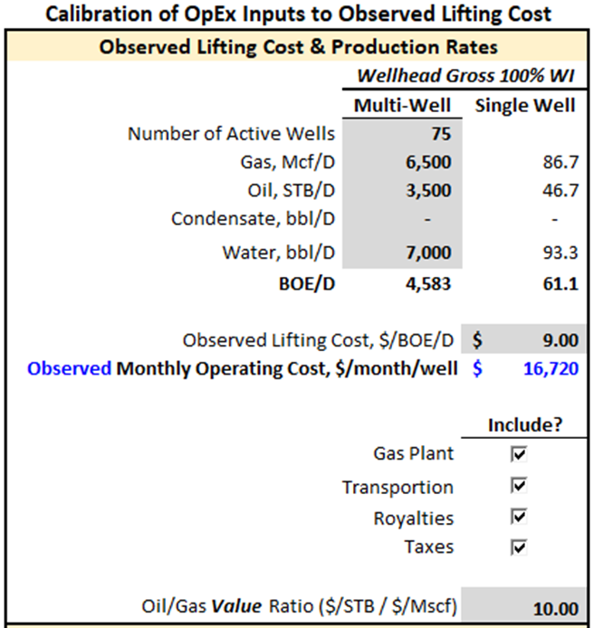
The production rates and lifting cost are entered in the “Inputs” tab in the grey shaded cells in the section shown below. The production rates can be single-well or multi-well. If multi-well, average single-well rates are computed and combined with the user-input lifting cost to compute an average single-well monthly operating costs. The check boxes in the picture below allow the user to include or exclude certain categories of costs in the model for the purpose of calibration. The royalty and taxes are converted to dollar amounts by inflating the other operating costs by 1/(1- royalty – taxes). This is necessary because commodity prices are not an input in this model. The Oil/Gas Value Ratio is used to production weight the overall severance tax %.
Once the observed data is entered, the user edits the numbers in the grey shaded cells in an iterative process to minimize the difference between the observed and model monthly operating costs. Economic Input items with a “Yes” in the “Lift Cost?” column will influence the monthly operating cost. Usually, the user will be altering the fixed and variable inputs in the Operating Cost section. There are inputs in other sections that impact monthly operating costs, but they may be known values, such as severance and ad valorem taxes, that would not be subject to change during calibration.
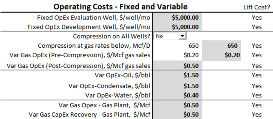
Pro Tip: Fixed OpEx and the Variable OpEx of the primary producing phase are often the most material variables to adjust for calibration. Enter reasonable values for all itmes with a 'Yes' Lift Cost and try adjusting only the Fixed OpEx and primary producing phase variable OpEx to achieve the calibration.
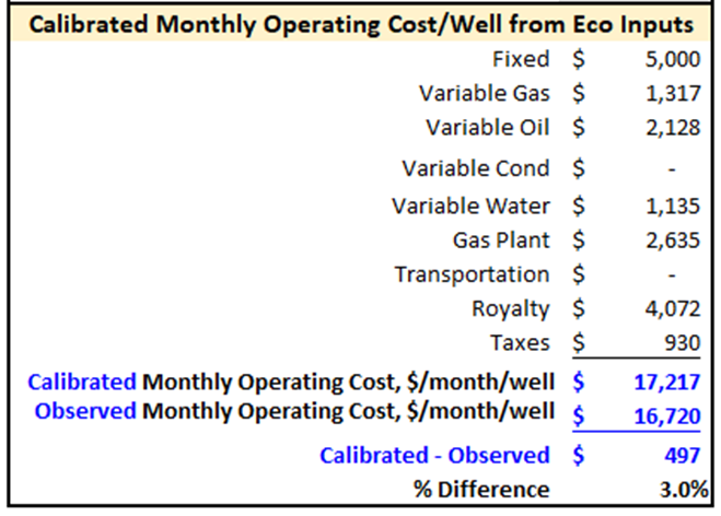
As the user iterates on the operating costs, the model vs observed error can be viewed in the “Inputs” tab in the section below.
Calibrate The NGL Model
The NGL model calibration typically amounts to choosing a model type, choosing a plant type, and entering any related inputs required from those choices. The results of the calibration are NGL component yields for Ethane, Butane, Propane, and Pentane +; the sales gas heating value, and the gas shrinkage due to NGL extraction and burning natural gas as fuel for the processing plant.
When turned on the model offers three options to compute NGL yields, gas shrinkage, and sales gas heating value with increasing degrees of sophistication. These models are selected from the “NGL’s Computed From” dropdown list:
- User Inputs
- User Inputs + Plant Type:
- Gas Analysis + Plant Type
There are six Plant Types to choose from, each with their own component extraction efficiencies:
- Dry Gas (no NGL extraction)
- Dew Point (gas chilled to roughly -9 C)
- Shallow Cut (gas chilled to roughly – 20 C)
- Deep Cut (gas chilled to roughly -100 C)
- Deep Cut X2 (w/ethane rejection)
- Custom (user defined component extraction efficiencies)
Pro Tip: If uncertain which NGL model to use, choose the more simple model.
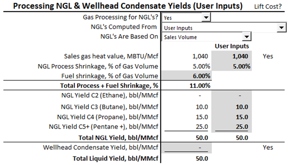
User Inputs Model:
This is the simplest NGL model and the user enters these items:
- NGL purity product (component) yields
- Sales gas heating value
- Process shrinkage and fuel shrinkage.
User Inputs + Plant Type Model:
This model requires the user to input several items in the “Inputs” tab:
- Theoretical NGL component yields (100% extraction efficiency)
- Observed total NGL yield
- Select a Plant Type
- Sales gas heating value
- Gas shrinkage % due to process (NGL extraction) and fuel usage
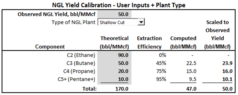
The theoretical yields are multiplied by the extraction efficiencies and then scaled to match the observed total NGL yield.
The plant type dictates the component extraction efficiencies which are only approximate. Actual plant efficiencies vary considerably. The user can enter specific extraction efficiencies in the “NGL Calculator” tab in the grey shaded cells as shown below. Select “Custom” as the plant type to use those user-entered efficiencies.

Any calibration effort usually involves confirming the observed total NGL yield and editing the “Custom” extraction efficiencies. The resulting NGL inputs are shown on the “Inputs” tab.
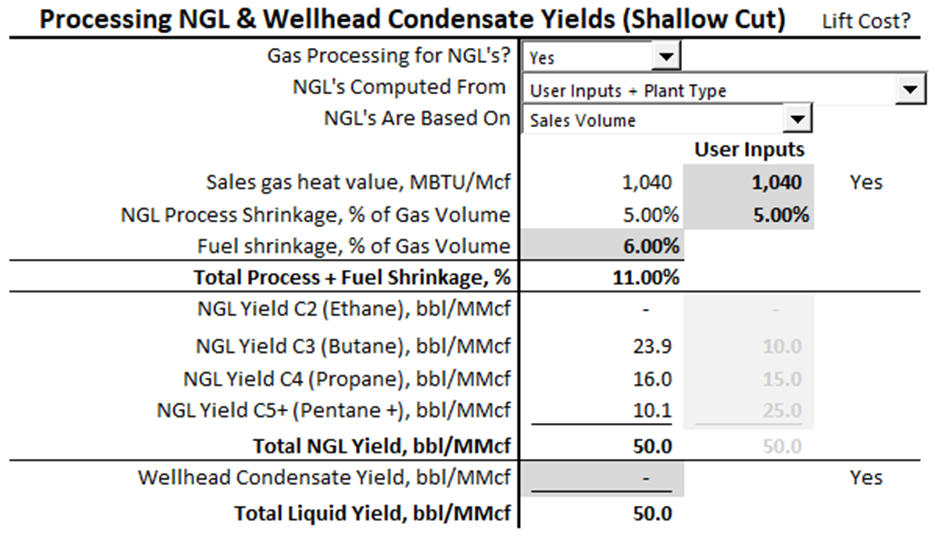
Gas Analysis + Plant Type Model
This is the most sophisticated of the three NGL models and requires several items:
- a gas analysis measuring the mole fraction of various components
- Select a Plant Type
- Gas shrinkage due to fuel usage
The gas analysis mole fractions are entered in the “NGL Calculator” tab shown below. These mole fractions determine the theoretical component yields, and when combined with the plant extraction efficiencies determine the realized component yields. This model also computes sale gas heating value and process shrinkage.
This model is not an Equation of State (EOS) model, but is a reasonable approximation of EOS model results.
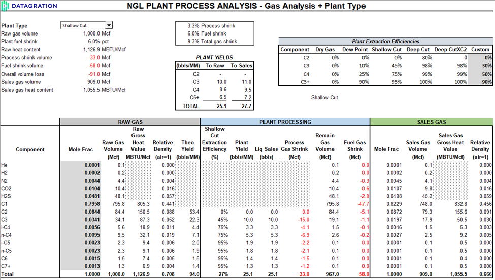
Any calibration effort usually involves editing the “Custom” extraction efficiencies. The resulting calibrated NGL inputs are found in the “Inputs” tab.
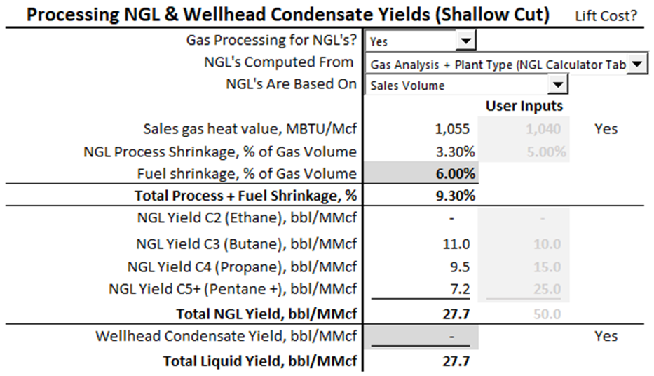
Enter The Economic Inputs Into PetroVisor
Once the user is satisfied with the results of the Economic Input Tool, the results can be input into PetroVisor.
First, confirm two economics-related Workspace Values are set for Completion Optimization. These should be set as part of the initial deployment of the Completion Optimization workflows.
Navigate to Workspace Settings by clicking on the gear icon next to the workspace name.

In the pop-up window that appears:
- 1. Enter "economic" in the search bar
- Confirm/Update:
- 2. EconomicsHierarchyName is set to Completion Optimization Design Cases
- 3. EconomicsParentEntityType is set to Economics

Note: If running other economic workflows (not Completion Optimization), the workspace values must be reset back to values required for the other workflows.
Enter/Edit Economic Inputs
View/edit the economic input values using a Data View.
- 1. Select the 'Data' menu item.
- 2. Select the 'Economics Parent Static Signals' Data View.
- 3. The economic inputs table will appear where they can be reviewed and edited.

From the PetroVisor Eco Inputs tool, find the variable for each header column and manually enter it in the Data View. There are more variables than shown in the graphic below.
- 1. Enter/edit values as needed
- 2. Select the 'Save Data' button when done to save changes.

Enter/Edit Commodity Prices
PetroVisor stores these monthly Commodity Prices:
- Hub Oil Price
- Hub Gas Price
- Condensate and NGL prices are stored as a % of the Hub OIl Price:
- Condenstate
- Ethane
- Butane
- Propane
- Pentane+
Pro Tip: If NGL's are being sold as a combined product (not fractionated), then impose the combined product commodity price for each of the purity product commodity prices, OR enter the combined NGL yield and commodity price in either the 'Condensate' phase or 'Pentanes+' phase.
To view/edit the Commodity Prices:
- 1. Select the 'Data' menu item.
- 2. Select the 'Economic Hub Prices' Data View.
- 3. Select the 'Date' menu item:
- 4. A pop-up window will appear. Change the beginning and ending dates as needed.
- 5. If the dates changed, they new date range can be seved by selecting the 'Save Data View' button.

- 6. Enter/Edit the commodity prices as needed. A cell can be copied across all the entire data range using Ctl-C on the cell to copy, highlighting the 'copy to' range, and using Ctl-V to paste the value.
- 7. Save changes by selecting the 'Save Data' button.
